We’ll be answering the following questions along the way:
1.) What was the change in price of the stock over time?
2.) What was the daily return of the stock on average?
3.) What was the moving average of the various stocks?
4.) What was the correlation between different stocks'?
5.) How much value do we put at risk by investing in a particular stock?
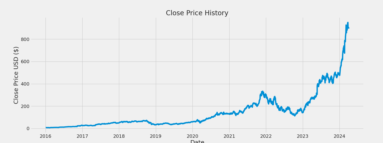
6.) How can we attempt to predict future stock behavior? (Predicting the closing price stock price of NVDA using LSTM)
Imports and Config
!pip install -q yfinance
import pandas as pd
import numpy as np
import matplotlib.pyplot as plt
import seaborn as sns
from pandas_datareader.data import DataReader
from pandas_datareader import data as pdr
import yfinance as yf
from datetime import datetime
from keras.models import Sequential
from keras.layers import Dense, LSTM

sns.set_style('whitegrid')
plt.style.use("fivethirtyeight")
%matplotlib inline
yf.pdr_override()
1. What was the change in price of the stock overtime?
# The tech stocks we'll use for this analysis
tech_list = ['AAPL', 'GOOG', 'MSFT', 'AMZN', "META", "NVDA", "TSLA"]

end = datetime.now()
start = datetime(end.year - 1, end.month, end.day)

for stock in tech_list:
    globals()[stock] = yf.download(stock, start, end)


company_list = [AAPL, GOOG, MSFT, AMZN, META, NVDA, TSLA]
company_name = ["APPLE", "GOOGLE", "MICROSOFT", "AMAZON", "META", "NVIDIA", "TESLA"]

for company, com_name in zip(company_list, company_name):
    company["company_name"] = com_name

df = pd.concat(company_list, axis=0)
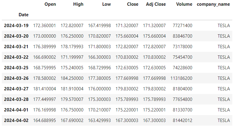
df.tail(10)
Descriptive Statistics about the Data
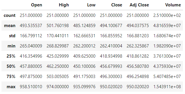
# Summary Stats
NVDA.describe()
Information About the Data
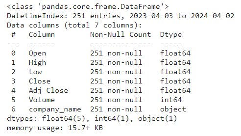
# General info
NVDA.info()
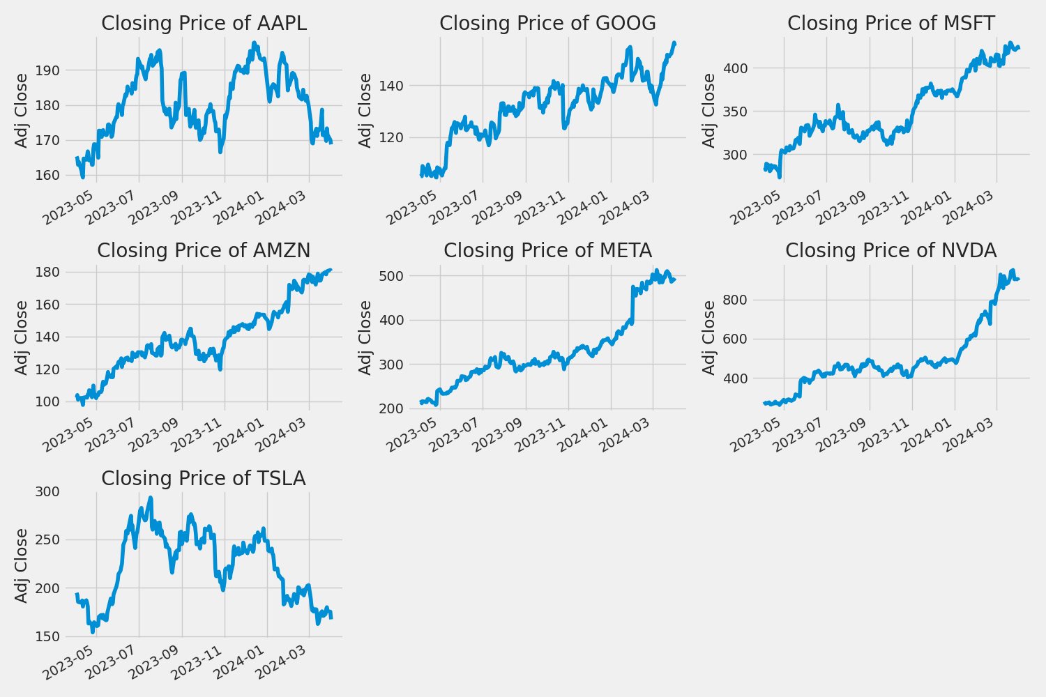
Closing Price
The closing price is the last price at which the stock is traded during the regular trading day.
plt.figure(figsize=(15, 10))
plt.subplots_adjust(top=1.25, bottom=1.2)

for i, company in enumerate(company_list, 1):
    plt.subplot(3, 3, i)
    company['Adj Close'].plot()
    plt.ylabel('Adj Close')
    plt.xlabel(None)
    plt.title(f"Closing Price of {tech_list[i - 1]}")

plt.tight_layout()
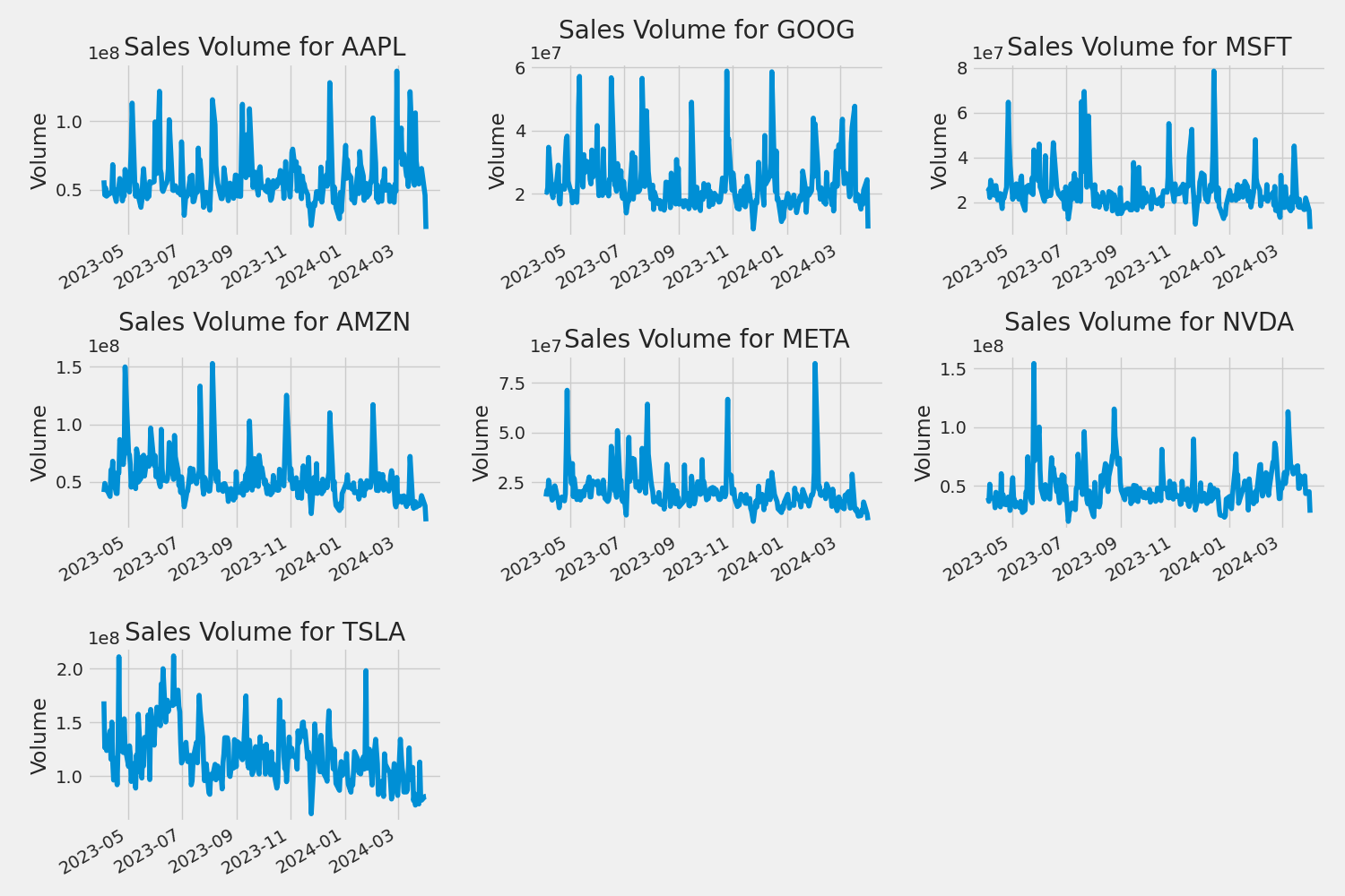
Volume of Sales
Volume is the amount of an asset or security that changes hands over some period of time, often over the course of a day.
plt.figure(figsize=(15, 10))
plt.subplots_adjust(top=1.25, bottom=1.2)

for i, company in enumerate(company_list, 1):
    plt.subplot(3, 3, i)
    company['Volume'].plot()
    plt.ylabel('Volume')
    plt.xlabel(None)
    plt.title(f"Sales Volume for {tech_list[i - 1]}")

plt.tight_layout()
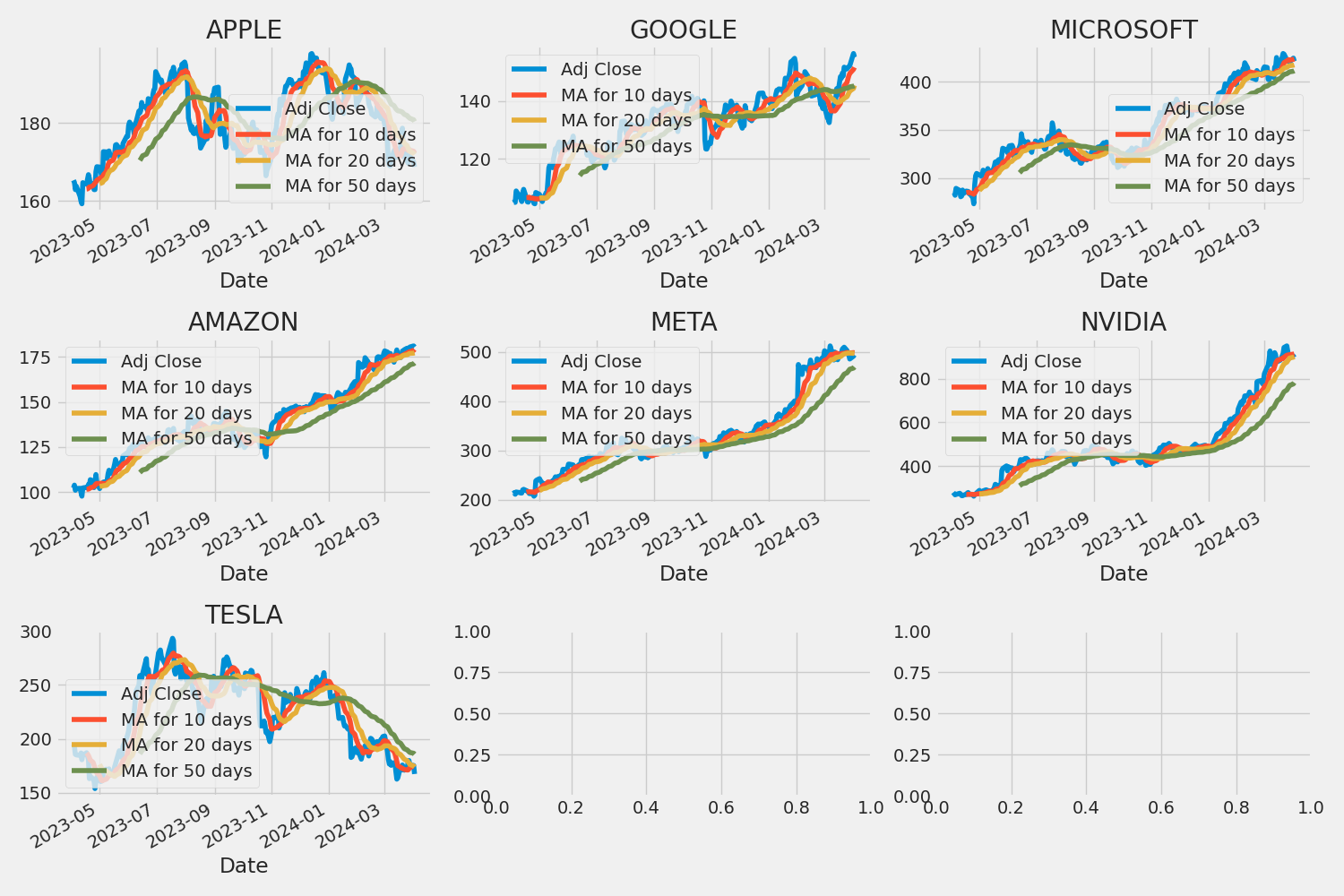
2. What was the moving average of the various stocks?
The moving average (MA) is a simple technical analysis tool that smooths out price data by creating a constantly updated average price.
ma_day = [10, 20, 50]

for ma in ma_day:
    for company in company_list:
        column_name = f"MA for {ma} days"
        company[column_name] = company['Adj Close'].rolling(ma).mean()

fig, axes = plt.subplots(nrows=3, ncols=3)
fig.set_figheight(10)
fig.set_figwidth(15)

AAPL[['Adj Close', 'MA for 10 days', 'MA for 20 days', 'MA for 50 days']].plot(ax=axes[0,0])
axes[0,0].set_title('APPLE')

GOOG[['Adj Close', 'MA for 10 days', 'MA for 20 days', 'MA for 50 days']].plot(ax=axes[0,1])
axes[0,1].set_title('GOOGLE')

MSFT[['Adj Close', 'MA for 10 days', 'MA for 20 days', 'MA for 50 days']].plot(ax=axes[0,2])
axes[0,2].set_title('MICROSOFT')

AMZN[['Adj Close', 'MA for 10 days', 'MA for 20 days', 'MA for 50 days']].plot(ax=axes[1,0])
axes[1,0].set_title('AMAZON')

META[['Adj Close', 'MA for 10 days', 'MA for 20 days', 'MA for 50 days']].plot(ax=axes[1,1])
axes[1,1].set_title('META')

NVDA[['Adj Close', 'MA for 10 days', 'MA for 20 days', 'MA for 50 days']].plot(ax=axes[1,2])
axes[1,2].set_title('NVIDIA')

TSLA[['Adj Close', 'MA for 10 days', 'MA for 20 days', 'MA for 50 days']].plot(ax=axes[2,0])
axes[2,0].set_title('TESLA')

fig.tight_layout()
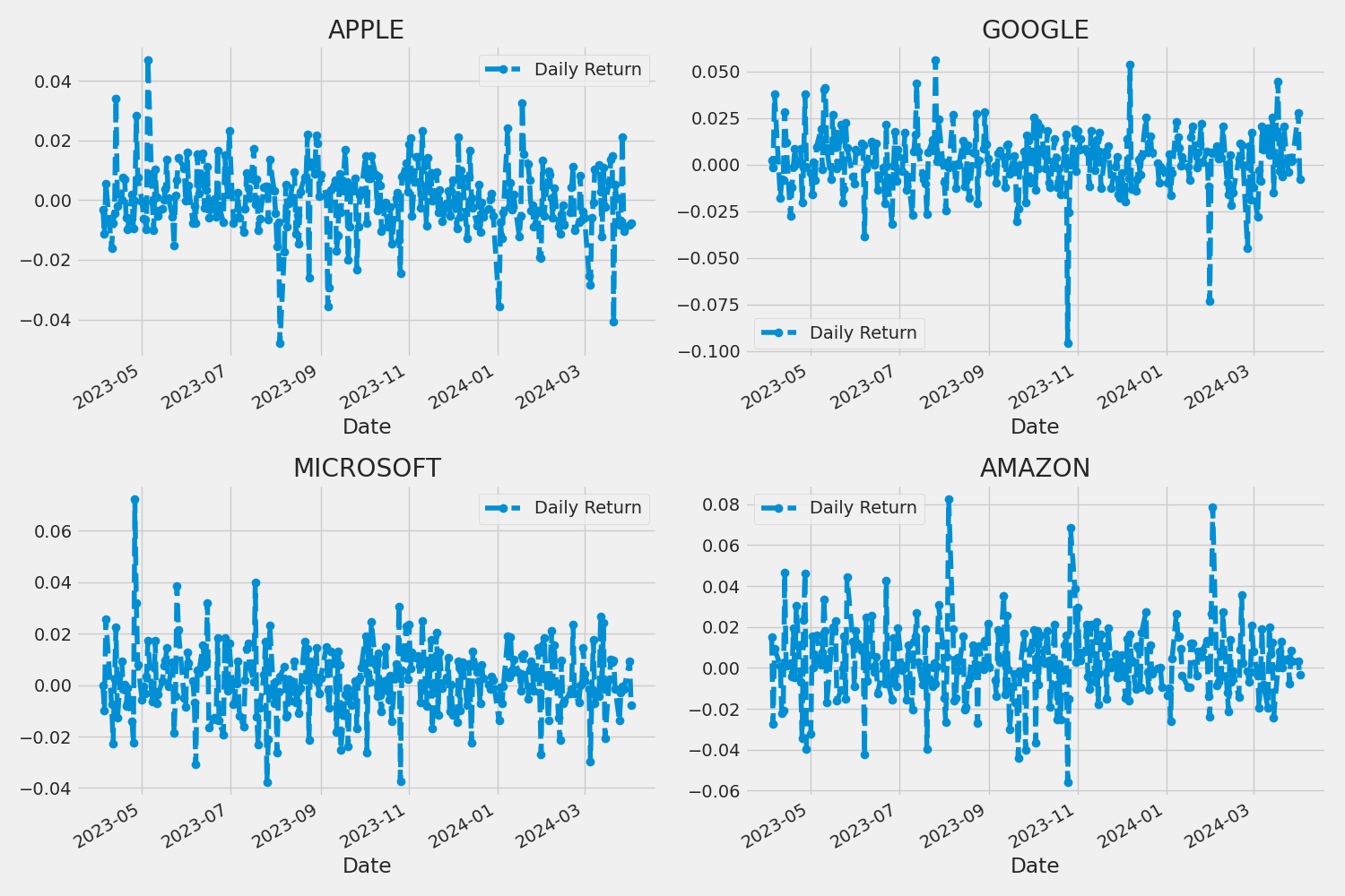
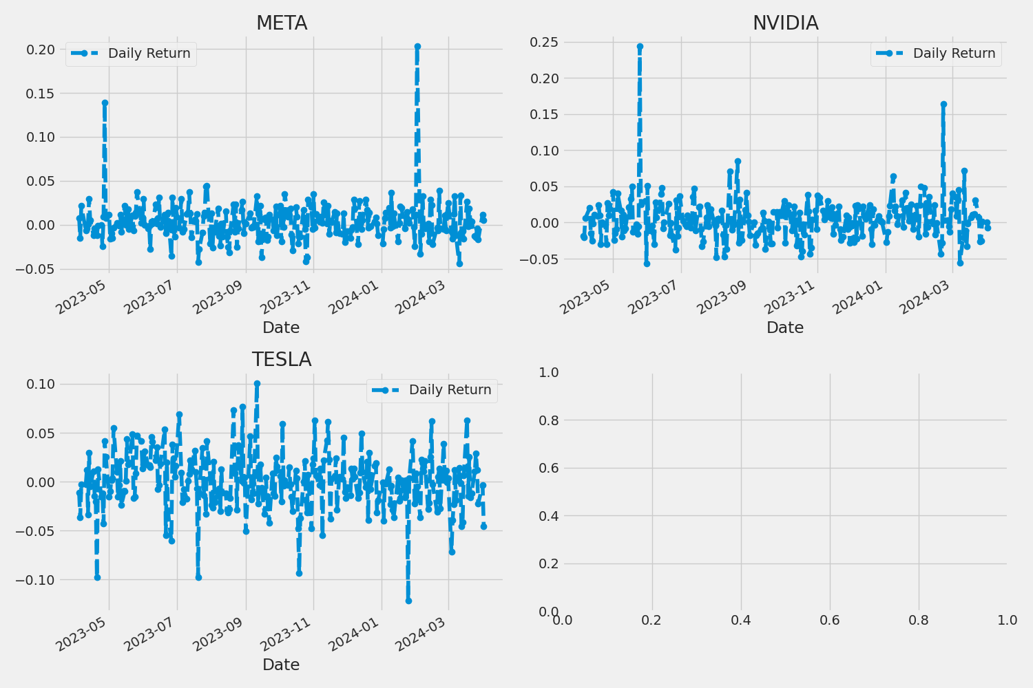
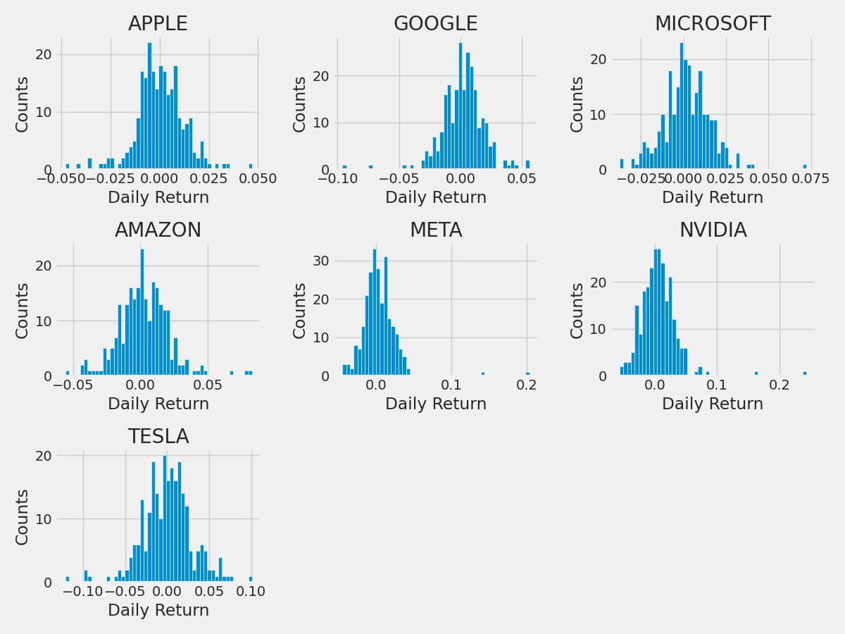
3. What was the daily return of the stock on average?
for company in company_list:
    company['Daily Return'] = company['Adj Close'].pct_change()

fig, axes = plt.subplots(nrows=2, ncols=2)
fig.set_figheight(10)
fig.set_figwidth(15)

AAPL['Daily Return'].plot(ax=axes[0,0], legend=True, linestyle='--', marker='o')
axes[0,0].set_title('APPLE')

GOOG['Daily Return'].plot(ax=axes[0,1], legend=True, linestyle='--', marker='o')
axes[0,1].set_title('GOOGLE')

MSFT['Daily Return'].plot(ax=axes[1,0], legend=True, linestyle='--', marker='o')
axes[1,0].set_title('MICROSOFT')

AMZN['Daily Return'].plot(ax=axes[1,1], legend=True, linestyle='--', marker='o')
axes[1,1].set_title('AMAZON')

fig.tight_layout()
for company in company_list:
    company['Daily Return'] = company['Adj Close'].pct_change()

fig, axes = plt.subplots(nrows=2, ncols=2)
fig.set_figheight(10)
fig.set_figwidth(15)

META['Daily Return'].plot(ax=axes[0,0], legend=True, linestyle='--', marker='o')
axes[0,0].set_title('META')

NVDA['Daily Return'].plot(ax=axes[0,1], legend=True, linestyle='--', marker='o')
axes[0,1].set_title('NVIDIA')

TSLA['Daily Return'].plot(ax=axes[1,0], legend=True, linestyle='--', marker='o')
axes[1,0].set_title('TESLA')

fig.tight_layout()
plt.figure(figsize=(12, 9))

for i, company in enumerate(company_list, 1):
    plt.subplot(3, 3, i)
    company['Daily Return'].hist(bins=50)
    plt.xlabel('Daily Return')
    plt.ylabel('Counts')
    plt.title(f'{company_name[i - 1]}')

plt.tight_layout()
4. What was the correlation between different stocks closing prices?
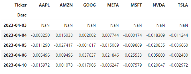
closing_df = pdr.get_data_yahoo(tech_list, start=start, end=end)['Adj Close']

# Make a new tech returns DataFrame
tech_rets = closing_df.pct_change()
tech_rets.head()
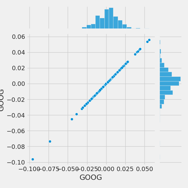
Now we can compare the daily percentage return of two stocks to check how correlated. First let’s see a sotck compared to itself.
# Comparing Google to itself should show a perfectly linear relationship
sns.jointplot(x='GOOG', y='GOOG', data=tech_rets, kind='scatter')
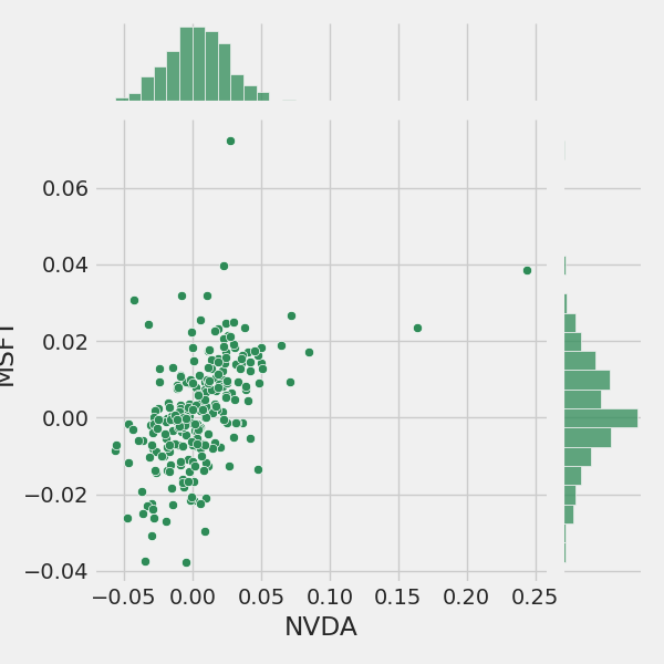
Correlation Between AI Companies and Nvidia
sns.jointplot(x='NVDA', y='MSFT', data=tech_rets, kind='scatter', color='seagreen')
sns.jointplot(x='NVDA', y='META', data=tech_rets, kind='scatter', color='seagreen')
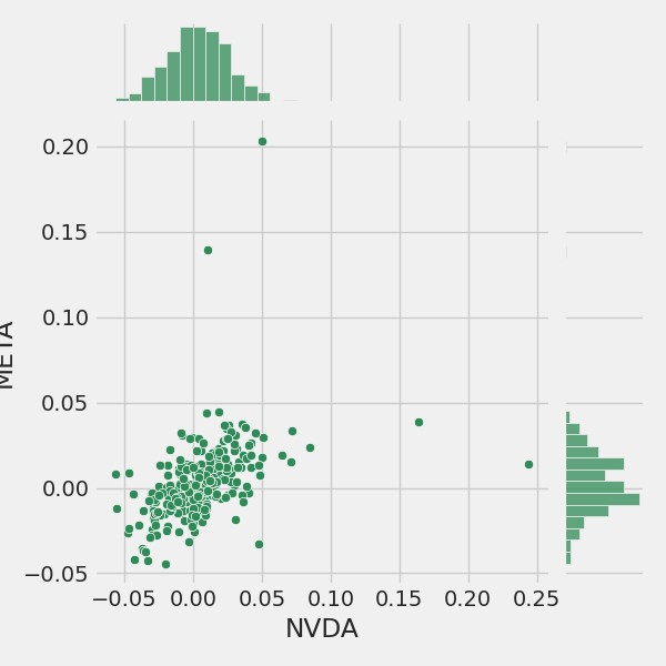
sns.jointplot(x='NVDA', y='AMZN', data=tech_rets, kind='scatter', color='seagreen')
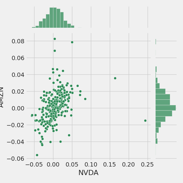
sns.jointplot(x='NVDA', y='GOOG', data=tech_rets, kind='scatter', color='seagreen')
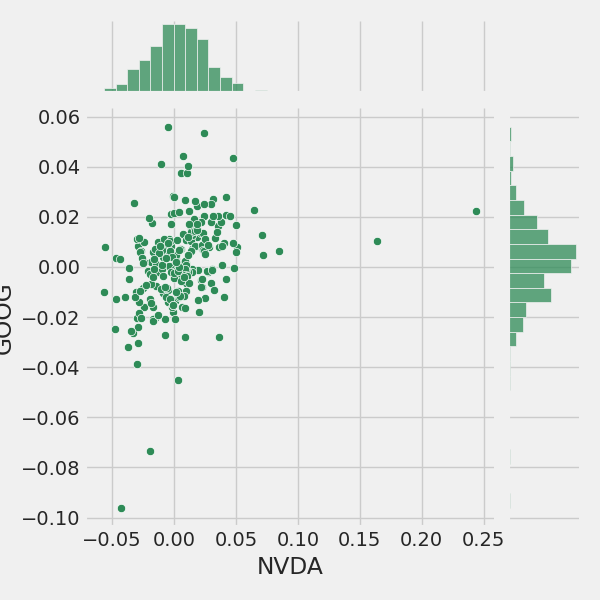
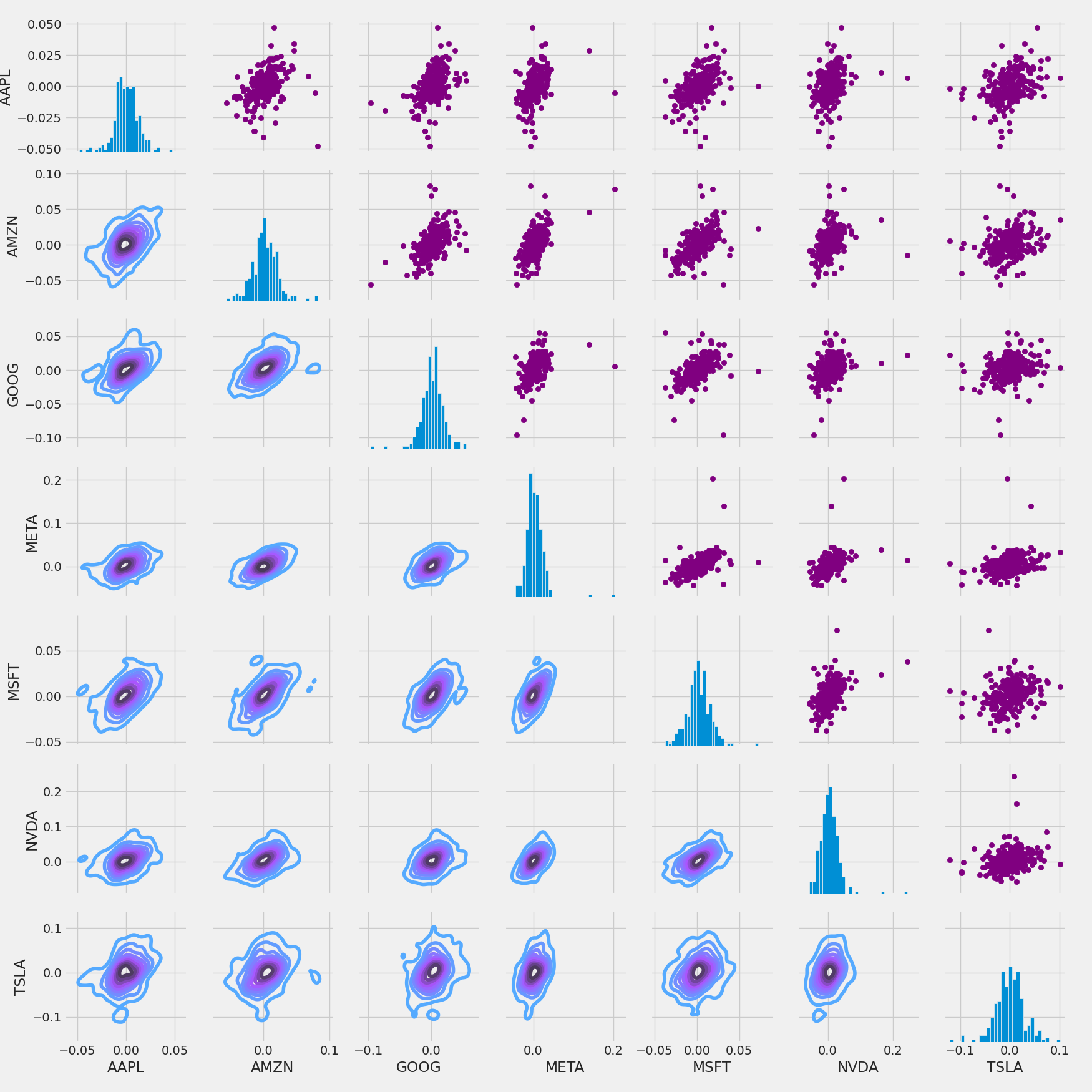
Returns Correlations
returns_fig = sns.PairGrid(tech_rets.dropna())

# Using map_upper we can specify what the upper triangle will look like.
returns_fig.map_upper(plt.scatter, color='purple')

# We can also define the lower triangle in the figure, inclufing the plot type (kde)
# or the color map (BluePurple)
returns_fig.map_lower(sns.kdeplot, cmap='cool_d')

# Finally we'll define the diagonal as a series of histogram plots of the daily return
returns_fig.map_diag(plt.hist, bins=30)
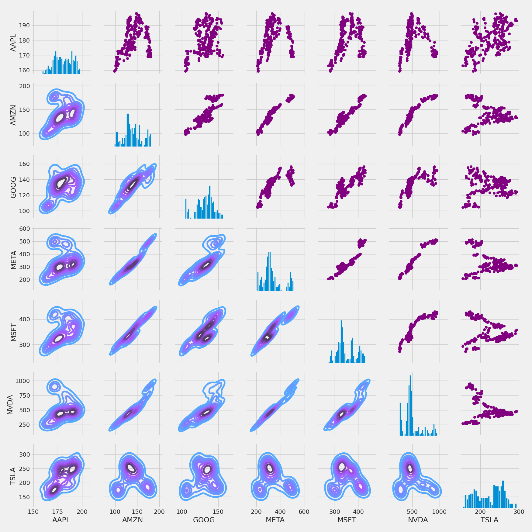
Closing Price Correlations
# Set up our figure by naming it returns_fig, call PairPLot on the DataFrame
closing_fig = sns.PairGrid(closing_df)

# Using map_upper we can specify what the upper triangle will look like.
closing_fig.map_upper(plt.scatter,color='purple')

# We can also define the lower triangle in the figure, inclufing the plot type (kde) or the color map (BluePurple)
closing_fig.map_lower(sns.kdeplot,cmap='cool_d')

# Finally we'll define the diagonal as a series of histogram plots of the daily return
closing_fig.map_diag(plt.hist,bins=30)
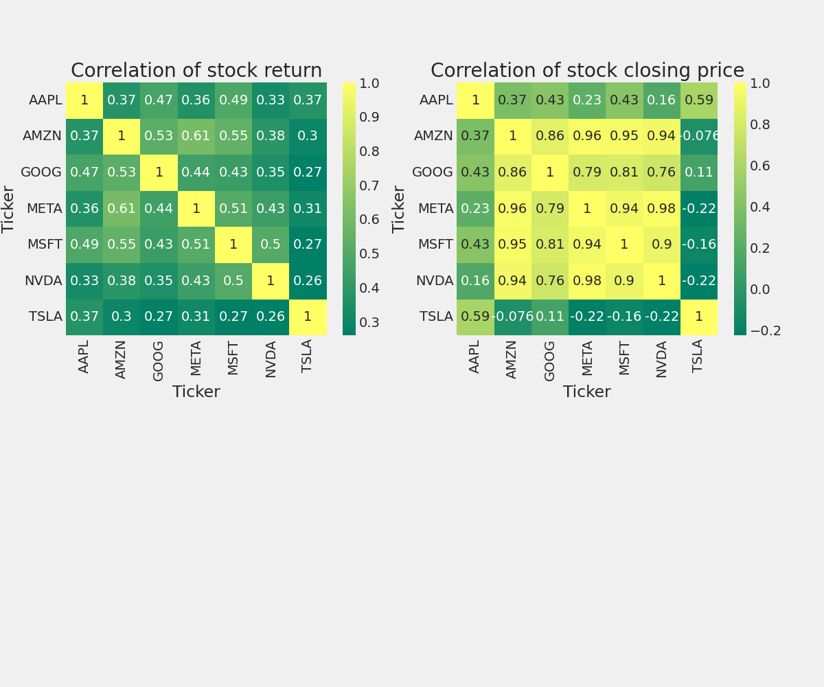
Correlation Matrix
plt.figure(figsize=(12, 10))

plt.subplot(2, 2, 1)
sns.heatmap(tech_rets.corr(), annot=True, cmap='summer')
plt.title('Correlation of stock return')

plt.subplot(2, 2, 2)
sns.heatmap(closing_df.corr(), annot=True, cmap='summer')
plt.title('Correlation of stock closing price')
5. How much value do we put at risk by investing in a particular stock?
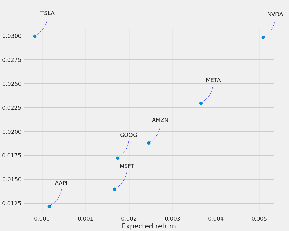
There are many ways we can quantify risk, one of the most basic ways using the information we’ve gathered on daily percentage returns is by comparing the expected return with the standard deviation of the daily returns.
rets = tech_rets.dropna()

area = np.pi * 20

plt.figure(figsize=(10, 8))
plt.scatter(rets.mean(), rets.std(), s=area)
plt.xlabel('Expected return')
plt.ylabel('Risk')

for label, x, y in zip(rets.columns, rets.mean(), rets.std()):
    plt.annotate(label, xy=(x, y), xytext=(50, 50), textcoords='offset points', ha='right', va='bottom',
                 arrowprops=dict(arrowstyle='-', color='blue', connectionstyle='arc3,rad=-0.3'))
6. Predicting the closing price stock price of NVDA:
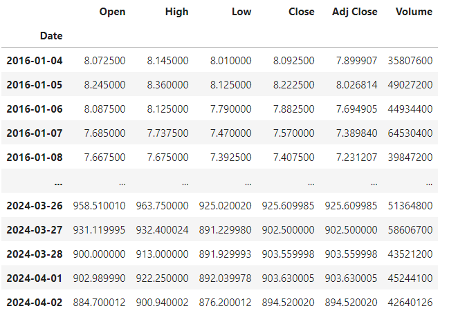
df = pdr.get_data_yahoo('NVDA', start='2016-01-01', end=datetime.now())
df
plt.figure(figsize=(16,6))
plt.title('Close Price History')
plt.plot(df['Close'])
plt.xlabel('Date', fontsize=18)
plt.ylabel('Close Price USD ($)', fontsize=18)
plt.show()
# Create a new dataframe with only the 'Close column
data = df.filter(['Close'])
# Convert the dataframe to a numpy array
dataset = data.values
# Get the number of rows to train the model on
training_data_len = int(np.ceil( len(dataset) * .95 ))

training_data_len
1972
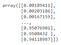
# Scale the data
from sklearn.preprocessing import MinMaxScaler

scaler = MinMaxScaler(feature_range=(0,1))
scaled_data = scaler.fit_transform(dataset)

scaled_data
train_data = scaled_data[0:int(training_data_len), :]
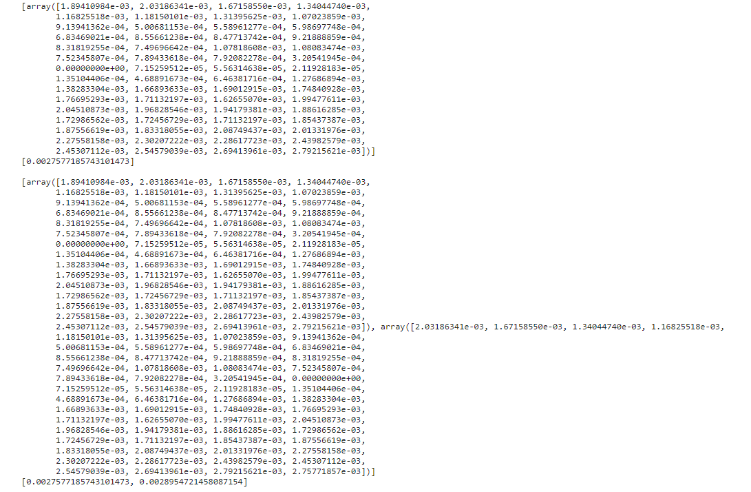
# Split the data into x_train and y_train data sets
x_train = []
y_train = []

for i in range(60, len(train_data)):
    x_train.append(train_data[i-60:i, 0])
    y_train.append(train_data[i, 0])
    if i<= 61:
        print(x_train)
        print(y_train)
        print()

# Convert the x_train and y_train to numpy arrays
x_train, y_train = np.array(x_train), np.array(y_train)

# Reshape the data
x_train = np.reshape(x_train, (x_train.shape[0], x_train.shape[1], 1))
# Build the LSTM model
model = Sequential()
model.add(LSTM(128, return_sequences=True, input_shape= (x_train.shape[1], 1)))
model.add(LSTM(64, return_sequences=False))
model.add(Dense(25))
model.add(Dense(1))

# Compile the model
model.compile(optimizer='adam', loss='mean_squared_error')

# Train the model
model.fit(x_train, y_train, batch_size=1, epochs=1)
# Create the testing data set
# Create a new array containing scaled values from index 1543 to 2002
test_data = scaled_data[training_data_len - 60: , :]
# Create the data sets x_test and y_test
x_test = []
y_test = dataset[training_data_len:, :]
for i in range(60, len(test_data)):
    x_test.append(test_data[i-60:i, 0])

# Convert the data to a numpy array
x_test = np.array(x_test)

# Reshape the data
x_test = np.reshape(x_test, (x_test.shape[0], x_test.shape[1], 1 ))

# Get the models predicted price values
predictions = model.predict(x_test)
predictions = scaler.inverse_transform(predictions)

# Get the root mean squared error (RMSE)
rmse = np.sqrt(np.mean(((predictions - y_test) ** 2)))
rmse
84.16346414984457
# Plot the data
train = data[:training_data_len]
valid = data[training_data_len:]
valid['Predictions'] = predictions
# Visualize the data
plt.figure(figsize=(16,6))
plt.title('Model')
plt.xlabel('Date', fontsize=18)
plt.ylabel('Close Price USD ($)', fontsize=18)
plt.plot(train['Close'])
plt.plot(valid[['Close', 'Predictions']])
plt.legend(['Train', 'Val', 'Predictions'], loc='lower right')
plt.show()
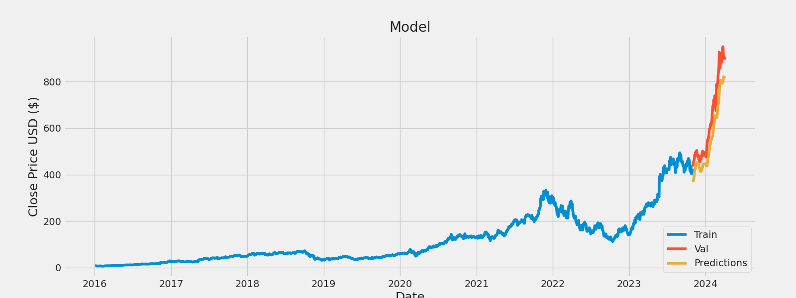
Predicting the exact value of a stock is challenging due to unpredictable market factors and information delays, making such predictions often outdated. Instead, forecasting the general direction of a stock, whether it will rise or fall, proves more reliable, considering the inherent uncertainties in market movements and providing valuable insights for investors.